
Niobium HSLA HAZ Toughness
A single weld thermal cycle that peaks at 1400 °C coarsens the prior austenite grains in the heat affected zone, and the microstructure it leaves behind is usually the weakest part of a welded joint. This study runs eleven experimental C-Mn steels through one such cycle, three carbon levels crossed with three niobium levels plus two manganese variants at a fixed niobium content, and then relates the Charpy results to two measured features of the microstructure, the area fraction of grain boundary ferrite and the area fraction of martensite-austenite constituent. The dividing line the work reports is a grain boundary ferrite fraction of about 6%. Above that figure the brittle fracture starts in the boundary ferrite, below it the fracture starts at the intersections of the bainitic packets.
Eleven experimental steels on one weld cycle
The base composition is a plain C-Mn steel. Three groups share 1.5% manganese and carry 0.05, 0.10 and 0.15% carbon, and inside each group three steels carry 0, 0.015 and 0.03% niobium. That gives carbon equivalents of 0.30, 0.35 and 0.40. Two further steels hold niobium at 0.015% and move the manganese instead, one to 2.1% and one to 0.9%, which separates the effect of manganese from the effect of niobium. The carbon equivalent is calculated as C plus Si divided by 24 plus Mn divided by 6 plus Ni divided by 40 plus Cr divided by 4 plus V divided by 14, in mass percent.
| Steel | C | Si | Mn | P | S | Al | Nb | N | Ceq |
|---|---|---|---|---|---|---|---|---|---|
| KT1 | 0.05 | 0.2 | 1.5 | 0.01 | 0.005 | 0.03 | 0 | 0.003 | 0.3 |
| KT2 | 0.05 | 0.2 | 1.5 | 0.01 | 0.005 | 0.03 | 0.015 | 0.003 | 0.3 |
| KT3 | 0.05 | 0.2 | 1.5 | 0.01 | 0.005 | 0.02 | 0.03 | 0.003 | 0.3 |
| KT4 | 0.1 | 0.2 | 1.5 | 0.01 | 0.005 | 0.02 | 0 | 0.003 | 0.35 |
| KT5 | 0.1 | 0.2 | 1.5 | 0.01 | 0.005 | 0.02 | 0.015 | 0.003 | 0.35 |
| KT6 | 0.1 | 0.2 | 1.5 | 0.01 | 0.005 | 0.02 | 0.03 | 0.003 | 0.35 |
| KT7 | 0.15 | 0.2 | 1.5 | 0.01 | 0.005 | 0.03 | 0 | 0.003 | 0.4 |
| KT8 | 0.15 | 0.2 | 1.5 | 0.01 | 0.005 | 0.02 | 0.015 | 0.003 | 0.4 |
| KT9 | 0.15 | 0.2 | 1.5 | 0.01 | 0.005 | 0.02 | 0.03 | 0.003 | 0.4 |
| KT10 | 0.05 | 0.2 | 2.1 | 0.01 | 0.005 | 0.02 | 0.015 | 0.003 | 0.4 |
| KT11 | 0.15 | 0.2 | 0.9 | 0.01 | 0.005 | 0.02 | 0.015 | 0.003 | 0.3 |
Source, Table 1 of the source chapter (PDF page 99). Chemical composition of the eleven steels in mass percent, with the carbon equivalent calculated from the formula printed in the chapter. The balance of every heat is iron.
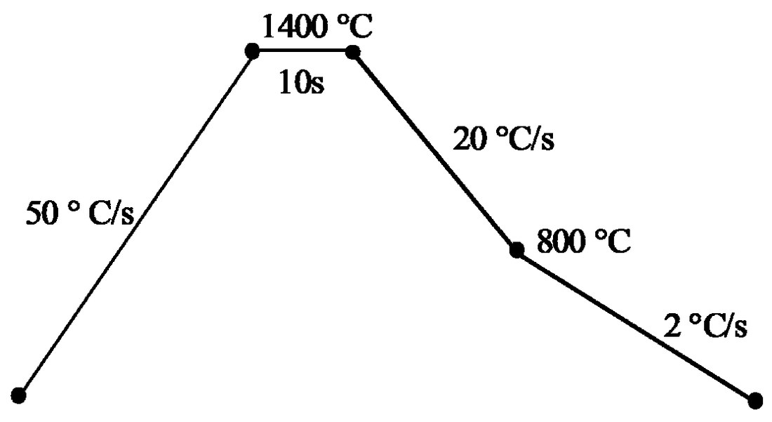
The cycle was chosen to produce the worst case rather than an average one, a single pass with a peak temperature of 1400 °C standing for a high heat input coarse grained HAZ. Heating runs at 50 °C per second to the peak, the hold lasts 10 seconds, cooling is 20 K per second between 1400 and 800 °C and then 2 K per second below 800 °C. Charpy specimens are 10 by 10 by 55 mm with the notch placed in the uniform microstructure at the centre of the specimen, and they were broken at 0, minus 20 and minus 40 °C to build the transition curves. Metallography used 2% nital and Le Pera etching, macro hardness was measured with a 10 kg load and micro hardness with a 10 g load, and the driving force for niobium carbide precipitation was calculated with Thermo-Calc.
Three microstructures the cycle can leave
Every simulated specimen is coarse grained, with grain boundary ferrite at the prior austenite boundaries and acicular ferrite inside the grains in the low niobium condition. Adding niobium shrinks the allotriomorphic ferrite layer and replaces the Widmanstatten ferrite with intragranular acicular ferrite, and at 0.03% niobium the acicular ferrite is itself replaced by a lath structure. Raising carbon at a fixed niobium content does the same thing, so the two additions act in the same direction on the transformation products.
The chapter groups the eleven results into three categories. Category I is the base steel with large areas of grain boundary ferrite, Widmanstatten ferrite and small areas of pearlite. Category II is a thin grain boundary ferrite layer plus intragranular acicular ferrite, and it covers the niobium free medium and high carbon steels together with the low carbon steel at medium niobium. Category III is a bainitic lath structure with a very thin and discontinuous boundary layer, and it covers the medium and high carbon equivalents with niobium plus the low carbon steel at high niobium. The point that matters for the rest of the page is that in category III not every grain boundary is covered by ferrite, and that discontinuity is what changes where a crack starts.
Niobium lowers the transformation temperature
Dilatometry records the temperature at which grain boundary ferrite starts to form during cooling, and the values fall as niobium rises in all three carbon groups. At a carbon equivalent of 0.30 the start temperature is 740 °C without niobium, 715 °C at 0.015% and 700 °C at 0.03%. At 0.35 the three values are 700, 670 and 660 °C, and at 0.40 they are 660, 640 and 630 °C. Carbon moves the same quantity down by a much larger step, about 40 °C between the 0.30 and the 0.35 groups.
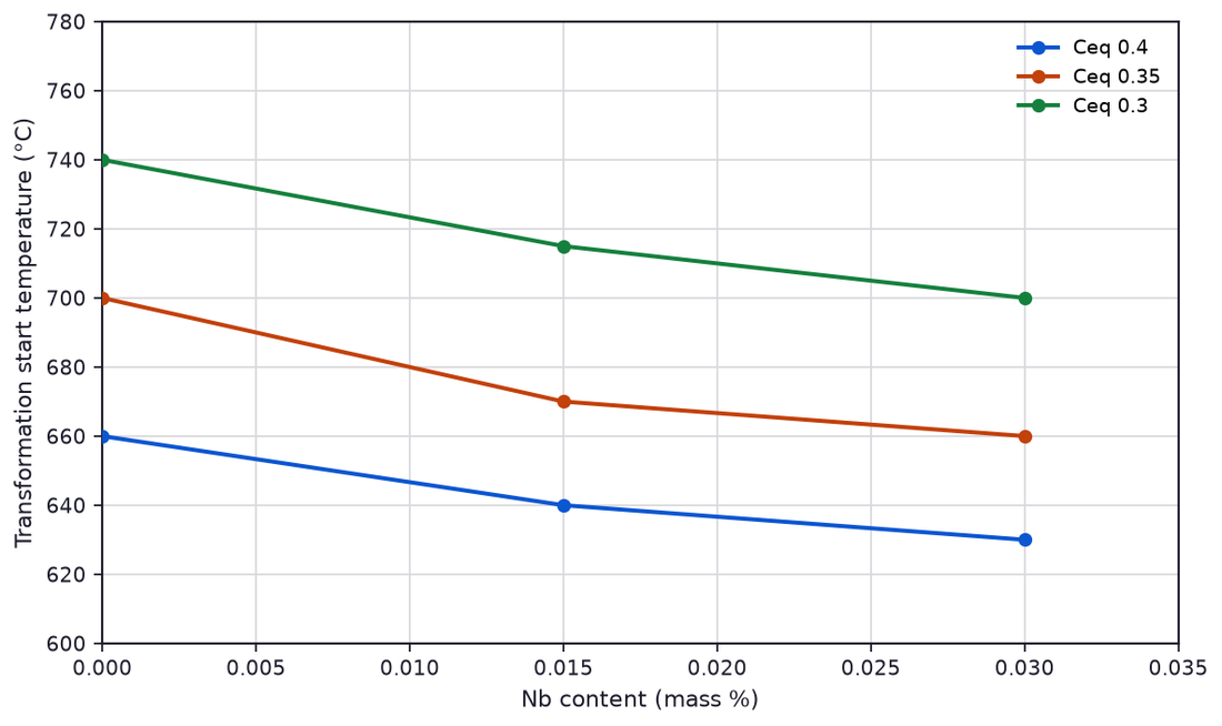
A lower start temperature means ferrite nucleation is delayed and the steel spends longer in the temperature range where bainite forms, which is exactly the microstructure change described above. The practical consequence is that niobium in the HAZ does not act only through grain refinement, which is its usual role in the parent plate, but also by suppressing the polygonal ferrite that would otherwise coat every prior austenite boundary.
Grain boundary ferrite and the martensite-austenite fraction
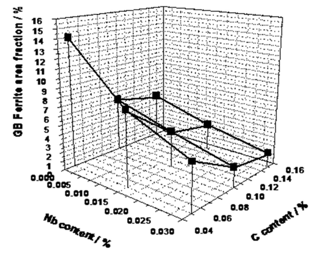
The area fractions were measured on the Le Pera etched specimens, and the two features move in opposite directions with niobium. The grain boundary ferrite falls steeply with niobium in the low carbon group and only slightly in the medium and high carbon groups, which the chapter attributes to niobium carbide precipitation consuming most of the niobium before it can segregate to the boundaries. Changing manganese or carbon within a carbon equivalent has little effect on the boundary ferrite fraction.
The martensite-austenite constituent, called MA throughout the chapter, rises with niobium in the low and medium carbon steels and does not rise in the high carbon steels, for the same reason. Where manganese moves at a fixed niobium content the effect is much larger than the niobium effect. At 2.1% manganese and a carbon equivalent of 0.40 the MA fraction reaches 5%, the highest in the series, and at 0.9% manganese at a carbon equivalent of 0.30 no MA was found at all, a result the authors confirmed on more than fifteen micrographs. That single comparison is the clearest statement in the chapter about which element governs MA.
Hardness and the Charpy transition curves
Hardness of the simulated HAZ rises with both carbon and niobium, in step with the change from ferrite to bainite described above. The transition behaviour separates the steels more sharply than hardness does. The lowest transition temperature belongs to KT4, a medium carbon steel with no niobium. KT2, the low carbon steel at 0.015% niobium, comes next, and KT11, the high carbon steel at low manganese, comes after it. Those three share a microstructure of grain boundary ferrite plus acicular ferrite and have closely similar hardness and grain size, which is why the acicular ferrite is credited with the better toughness in the chapter.
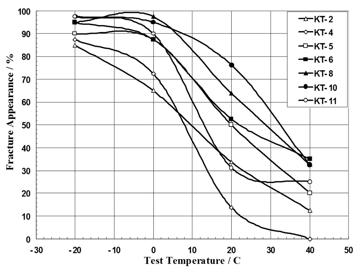
The two worst curves belong to KT8 and KT10, the two steels at the highest carbon equivalent of 0.40. KT10 carries the highest MA fraction in the series and KT8 one of the lowest, yet their transition curves sit almost on top of each other. The authors draw the conclusion directly, that the transition temperature is set by the microstructure features and not by the MA fraction, which is the point on which earlier work in this field disagreed.
Where the brittle fracture starts, and the 6% rule
Fracture surfaces were examined for all steels and the initiation site was classified against the microstructure at that point. Three categories came out. The base steel breaks at regenerated pearlite colonies near the prior austenite boundary, and the steels with a relatively large area of boundary ferrite break inside that ferrite. Where the boundary ferrite is thin and discontinuous the fracture starts at the intersection of bainitic packets with different orientation and propagates through the packets. The fracture unit was measured on the minus 40 °C specimens and came out at about 90 µm for every steel, so niobium does not change the size of the cleavage unit at these levels.
| Steel | C % | Ceq | Nb % | Grain size, µm | Microstructure | G.B. ferrite % | MA % | Initiation point |
|---|---|---|---|---|---|---|---|---|
| Low C, free Nb | 0.05 | 0.3 | 0 | 348 | Widmanstatten ferrite plus grain boundary ferrite plus small areas of pearlite | 14 | 0.2 | Regenerated pearlite near the grain boundary |
| Low C, Nb | 0.05 | 0.3 | 0.03 | 207 | Lath structure | 5 | 1 | Intersection of bainitic packets |
| Med. C, free Nb | 0.1 | 0.35 | 0 | 336 | Grain boundary ferrite plus Widmanstatten ferrite plus acicular ferrite | 6 | 0.5 | At the grain boundary |
| Med. C, Nb | 0.1 | 0.35 | 0.03 | 248 | Lath structure | 2 | 2 | Intersection of bainitic packets |
| High C, free Nb | 0.15 | 0.4 | 0 | 342 | Grain boundary ferrite plus Widmanstatten ferrite plus acicular ferrite | 6 | 0.5 | At the grain boundary |
| High C, Nb | 0.15 | 0.4 | 0.03 | 230 | Lath structure | 1.8 | 1 | Intersection of bainitic packets |
| Low C, high Mn | 0.05 | 0.4 | 0.015 | 236 | Lath structure | 2.5 | 5 | Intersection of bainitic packets |
| High C, low Mn | 0.15 | 0.3 | 0.015 | 330 | Grain boundary ferrite plus Widmanstatten ferrite plus acicular ferrite | 6 | 0 | At the grain boundary |
Source, Table 2 of the source chapter (PDF page 113). Grain size, microstructure, grain boundary ferrite fraction, MA fraction and the initiation site observed on specimens broken at minus 40 °C.
Reading the table by the boundary ferrite fraction rather than by composition gives a clean split. Every steel at 6% or more broke in the boundary ferrite or in the pearlite next to it, and every steel below 6% broke at a packet intersection. The physical reason the chapter gives is a hardness step, the boundary ferrite sits about 100 HV below the interior of the grain, so a continuous boundary layer concentrates stress and cracks there. Below 6% the layer no longer covers every grain, the matrix is mostly bainite with MA aligned along the laths, and the stress concentration moves to the packet boundaries.
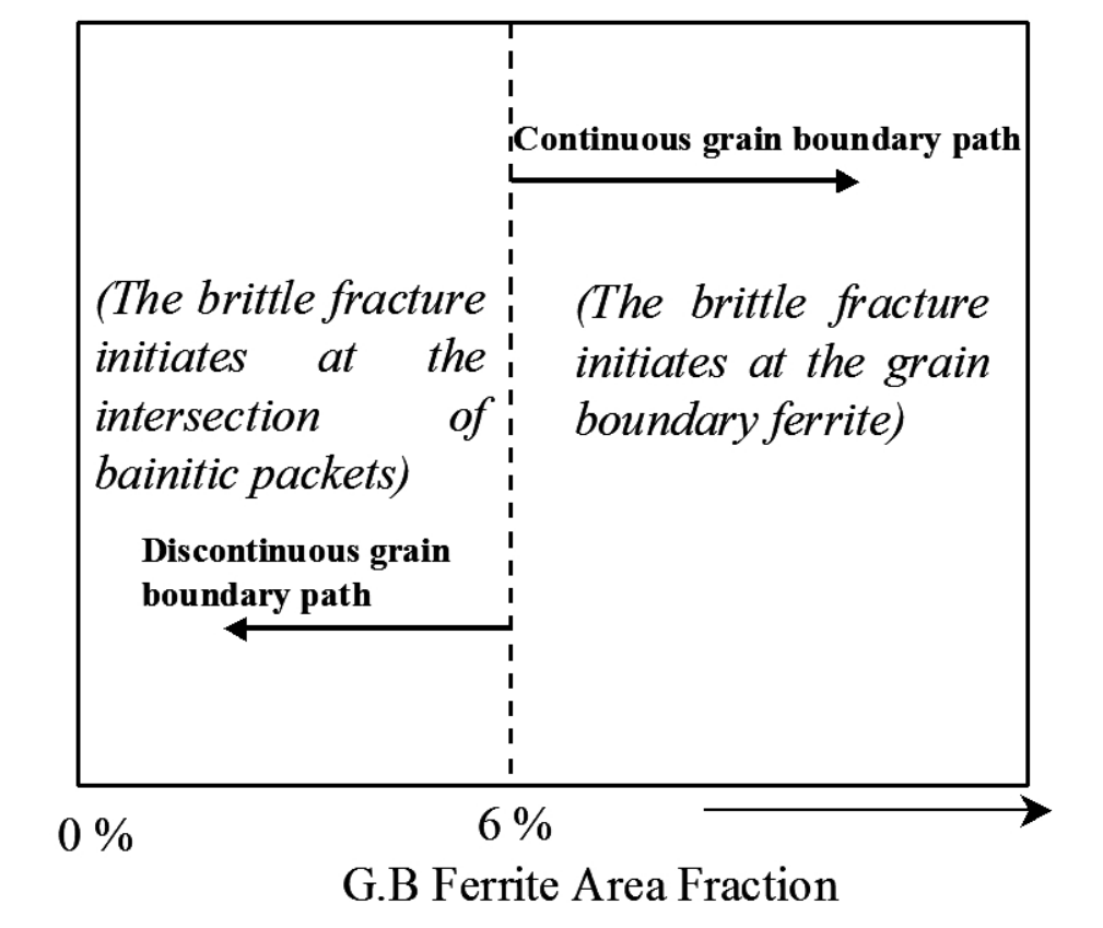
The chapter is careful about how far the 6% figure can travel. The boundary ferrite fraction depends on composition, on the thermal cycle and on the prior austenite grain size, so the number is a criterion for this family of steels under this cycle and not a universal threshold for every HSLA grade.
Why manganese decides the MA fraction
The proposed mechanism is that boundary ferrite rejects carbon and alloying elements into the austenite ahead of it as it grows, so the region between the ferrite and the bainite becomes enriched and partly transforms to MA on further cooling. Electron microprobe line scans across the simulated specimens confirm the enrichment. Carbon and manganese both segregate, and manganese segregates more strongly than carbon in the 2.1% manganese steel.
The 0.9% manganese steel is the test of the mechanism. It shows clear carbon enrichment at the boundary but only weak manganese segregation, and it contains no MA at all. The authors therefore require both conditions at once, carbon enrichment and alloying element segregation, and note that niobium itself showed no measurable segregation at 0.015%, too low a level for the probe to resolve. This explains why the manganese variants move the MA fraction further than niobium additions of the same order do, and why the steel at 2.1% manganese reaches the highest MA fraction in the series at 5%, against 0.2% in the 1.5% manganese base steel.
What this means for a steel order
The results give a buyer of HSLA plate three quantities to ask for when toughness of the welded joint is the requirement. The first is the carbon equivalent, because it sets both the transformation temperature and the amount of bainite in the coarse grained HAZ. The second is the manganese level relative to that carbon equivalent, because manganese is the element that decides whether MA forms at all. The third is a simulated HAZ Charpy result at the lowest service temperature rather than a parent plate result, since the parent plate properties say nothing about the coarse grained region next to the weld.
Niobium between 0.015 and 0.03% at 1.5% manganese is the condition that produced the fine bainitic structures with boundary ferrite under 6% in this work, and those steels broke at packet intersections rather than along the boundaries. The same niobium addition at 2.1% manganese produced the highest MA fraction and one of the two worst transition curves, so niobium on its own is not a toughness addition. For the metallurgical background of how niobium and titanium raise strength in the parent plate, see microalloyed steel strengthening mechanisms, and for the strip grades whose compositions these experimental heats are modelled on, see microalloyed strip steel compositions. The tempering behaviour of the same class of low alloy steel is covered on low alloy steel tempering kinetics.
Source: Alloy Steel, Properties and Use, InTech, 2011, Chapter 4, Tables 1 and 2 and Figures 1, 4, 8, 12 and 16 (PDF pages 99 to 113), licensed CC BY 3.0. The chapter reports work originally published in the references it cites. Every table and figure on this page was rendered from the source PDF at 300 dpi and read cell by cell before the text above was written, and the numbers were checked against the source text layer, with the rendered image taken as authoritative where the two differ. This page is a reference summary of published research and not an Aobo Steel specification, so confirm the grade and the weld procedure before the numbers are written into a process sheet.