
Low Alloy Steel Tempering Kinetics
When a quenched low alloy steel is tempered, two reactions run through it in sequence and partly overlap. A dilatometer records both of them as changes in the length of the specimen, and the curve can be separated into the two reactions and fitted to the Avrami formalism so that each one gets its own exponent, rate constant and activation energy. This page collects those parameters for two steels, a 0.32% carbon low alloy steel tempered isothermally at 350 °C, and AISI 1050 tempered at constant heating rates of 5 to 30 K per minute. For a tool steel, where the tempering response of a specific grade is what matters, the practical curves are on the tool steel tempering chart; this page is the reaction kinetics behind those curves.
The two processes a dilatometry curve shows
The steel used for the isothermal work contains 0.32% C, 1.12% Mn, 0.67% Si, 0.07% Ni, 0.02% P and 0.05% S, the balance iron. Specimens 9 mm in diameter and 100 mm long were austenitized at 900 °C for 30 minutes, quenched in water at ambient temperature, and then held at 350 °C in a dilatometer with a length resolution of 10-3 mm. Its martensite start temperature is about 365 °C, so the 350 °C hold sits just below Ms and the whole tempering sequence happens in one isothermal step.
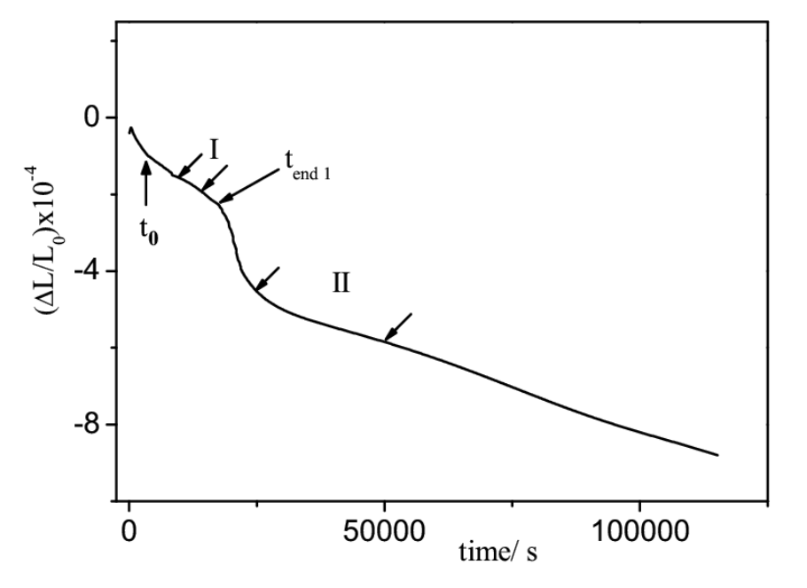
Two contractions appear in the length of the specimen. The first is the faster of the two and ends at t end 1, the second takes over after it and runs on to the end of the record. Each was fitted separately, using only a work interval well away from the start and the end of the reaction, and the fitted parameters are collected below.
| Parameter, first process | Value |
|---|---|
| Best interval in the experimental fraction transformed | 0.5050 to 0.7625 |
| Work interval in the first process fraction after the final iteration | 0.5310 to 0.7750 |
| N, slope of the linear fit | 1.58 |
| Correlation coefficient R for N | 0.993 |
| n1, Avrami exponent | 1.49 |
| Correlation coefficient R for n1 | 0.992 |
| k1, rate constant (s-1) | 1.2 x 10⁻⁴ |
Source, Table 10.b of the source chapter. Kinetic parameters for the first process on tempering of the 0.32% carbon low alloy steel, fitted by the method the source calls KTOPT.
| Parameter, second process | Value |
|---|---|
| Best interval in the experimental fraction transformed | 2.864 to 3.963 |
| Normalized interval in the transformed fraction | 0.4506 to 0.6544 |
| Work interval in the second process fraction after the final iteration | 0.5975 to 0.8010 |
| N, slope of the linear fit | -0.669 |
| Correlation coefficient R for N | 0.998 |
| n2, Avrami exponent | 0.669 |
| Correlation coefficient R for n2 | 0.998 |
| k2, rate constant (s-1) | 4.4 x 10⁻⁵ |
Source, Table 10.a of the source chapter. Kinetic parameters for the second process on the same steel and the same 350 °C hold.
The rate constants differ by a factor of about three, k1 at 1.2 x 10⁻⁴ per second and k2 at 4.4 x 10⁻⁵ per second, which is the quantitative statement of the first process being the faster one.
Which reaction each process is
The Avrami exponents identify the mechanisms, because the value of n is fixed by how a reaction nucleates and grows. An exponent of 1.5 corresponds to diffusion controlled growth from a fixed number of nuclei, that is, growth with a nucleation rate of zero, and that is the value returned for the first process. The first stage of tempering is the decomposition of martensite into a transition carbide and a less tetragonally distorted martensite, and the exponent is consistent with that reaction when it happens in a specimen that was already partly transformed during the quench. The study notes that the transition carbide may in part have formed before the 350 °C hold began, since Ms is about 365 °C.
An exponent of about 0.67 corresponds to precipitation on dislocations with diffusion controlled growth, for which the literature value is 0.66. The second process is the disappearance of the transition carbide and the formation of stable cementite, and cementite is reported to nucleate on dislocations and on lath and grain boundaries, which is exactly the mechanism that exponent describes. Applying the uncertainty in the measured fraction transformed to the exponents gives n1 of 1.5 with bounds of about 0.2, and n2 of 0.67 with bounds of about 0.02.
Non-isothermal tempering of AISI 1050
The second half of the work takes a different steel and a different thermal history. The steel is AISI 1050, with 0.48 to 0.55% C, 0.6 to 0.9% Mn, 0.04% P and 0.05% S, and it was heated from ambient temperature to 600 °C at constant rates of 5, 10, 15, 20 and 30 K per minute in a dilatometer with a resolution of 10-4. Plotting the rate of change of the relative length against temperature separates the two reactions into two bands, and the higher the heating rate, the further both bands move to the right.
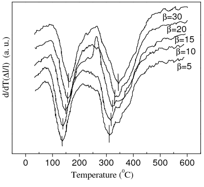
The temperature of the inflection point of each band, at each heating rate, is the raw input to the rest of the calculation. An inflection point is used rather than a peak because the analysis requires the point at which the second derivative of the fit is zero.
| β (K/min) | Ti (K), Process I | Ti (K), Process II |
|---|---|---|
| 5 | 411.6 | 584.3 |
| 10 | 418.9 | 593.5 |
| 15 | 424.3 | 599.1 |
| 20 | 428.5 | 603.1 |
| 30 | 432.4 | 608.8 |
Source, Table 11 of the source chapter. Temperatures corresponding to the inflection points at different heating rates, for the two processes on tempering of AISI 1050.
The shift is modest in absolute terms but consistent in direction. Raising the heating rate from 5 to 30 K per minute moves the first process from 411.6 to 432.4 K, a shift of about 21 K, and the second from 584.3 to 608.8 K, a shift of about 25 K. That displacement is the basis of every Kissinger-like method, because a reaction with a higher activation energy shifts further for the same change in heating rate.
Activation energy and frequency factor
Two routes to the activation energy are reported. A Kissinger-like plot uses only the temperatures at which a fixed fraction is transformed, and it returns the effective activation energy without any assumption about the reaction model. A second, non-linear regression route fits both the activation energy and the frequency factor at the same time. The results are set out below, and the two routes agree.
| Process | Activation energy E (kJ/mol) | Frequency factor K0 (min-1) | Confidence interval for E | Regression coefficient R | P value for E |
|---|---|---|---|---|---|
| I | 117 | 2.99 x 10¹⁴ | 104 to 130 (linear) | 0.998 | 4.8 x 10⁻¹⁰ |
| II | 206 | 9.53 x 10¹⁷ | 196 to 216 (linear) | 0.999 | 9.0 x 10⁻¹⁴ |
Source, Table 12 of the source chapter. Best parameters E and K0 calculated by linear and non-linear regression for the two processes on tempering of AISI 1050. The source also prints narrow non-linear confidence intervals, 116.5 to 117.4 kJ/mol for the first process and 205.6 to 206.4 kJ/mol for the second, and gives the P value as the probability that another model fits the same data better.
The first process needs 117 kJ/mol and the second 206 kJ/mol. The second value sits in the range normally quoted for the diffusion of carbon in ferrite and for the coarsening of cementite, which is consistent with the mechanism assigned to it above. The frequency factors span three orders of magnitude between the two processes, and the two values are printed here as the source gives them.
The Avrami exponent at each heating rate
The same non-isothermal records also yield the Avrami exponent, but the authors take it from a transcendental equation rather than from the regression used above, because they consider the regression route too sensitive to the approximations behind it. The exponents and their uncertainties are given per heating rate.
| First process on tempering | |||
|---|---|---|---|
| β (K/min) | Ti (K) | n | δn |
| 5 | 411.6 | 1.2 | 0.2 |
| 10 | 418.9 | 1.1 | 0.2 |
| 15 | 424.3 | 1.0 | 0.2 |
| 20 | 428.5 | 1.1 | 0.2 |
| 30 | 432.4 | 1.0 | 0.2 |
| Second process on tempering | |||
|---|---|---|---|
| β (K/min) | Ti (K) | n | δn |
| 5 | 584.3 | 0.7 | 0.1 |
| 10 | 593.5 | 0.7 | 0.1 |
| 15 | 599.1 | 0.7 | 0.1 |
| 20 | 603.1 | 0.7 | 0.1 |
| 30 | 608.8 | 0.7 | 0.1 |
Source, Table 13 of the source chapter. The Avrami exponent for the two processes on tempering of AISI 1050 at each heating rate, with the uncertainty calculated from the uncertainty in temperature and in activation energy. The two frames are the source’s own division of one table, first process above and second process below.
The first process scatters between 1.0 and 1.2 with a stated uncertainty of 0.2 on every row, so the values are not distinguishable from one another, and the mean sits close to the 1.5 obtained isothermally once the uncertainty is taken into account. The second process is constant at 0.7 to within 0.1 at every heating rate, which is the same exponent the isothermal fit returned.
Activation energy and frequency factor at each heating rate
Fixing the exponent permits the frequency factor to be calculated for each heating rate separately, and the resulting activation energies can be compared with the single value from the Kissinger-like plot above.
| β (K/min) | Ti (K) | n0 | K0 (min-1) | E (kJ/mol) | δE (kJ/mol) |
|---|---|---|---|---|---|
| 5 | 411.6 | 1.0 | 5.4 x 10¹⁴ | 119 | 6 |
| 10 | 418.9 | 1.0 | 6.87 x 10¹³ | 112 | 6 |
| 15 | 424.3 | 1.0 | 3.3 x 10¹⁴ | 117 | 6 |
| 20 | 428.5 | 1.0 | 2.0 x 10¹⁵ | 124 | 7 |
| 30 | 432.4 | 1.0 | 1.1 x 10¹⁴ | 113 | 6 |
Source, Table 14 of the source chapter. Activation energies and frequency factors for the first process on tempering of AISI 1050, calculated for each heating rate from the inflection point temperature with the exponent n0 fixed at 1.0.
| β (K/min) | Ti (K) | n0 | K0 x 1017 (min-1) | E (kJ/mol) | δE (kJ/mol) |
|---|---|---|---|---|---|
| 5 | 584.3 | 1.4 | 1.3 | 196 | 11 |
| 10 | 593.5 | 1.4 | 1.2 | 196 | 10 |
| 15 | 599.1 | 1.4 | 1.3 | 196 | 10 |
| 20 | 603.1 | 1.4 | 1.6 | 197 | 10 |
| 30 | 608.8 | 1.4 | 1.3 | 196 | 10 |
Source, Table 15 of the source chapter. Activation energies and frequency factors for the second process on tempering of AISI 1050, with the exponent n0 fixed at 1.4. The frequency factor column is printed by the source in units of 1017 per minute, while the activation energy is given per mol.
The second process is the more reproducible of the two. Its activation energy is 196 to 197 kJ/mol at every heating rate, inside the error bound of about 10 kJ/mol, and the frequency factor varies by less than a factor of 1.4 across a sixfold change in heating rate. The first process scatters more, from 112 to 124 kJ/mol, which is what an exponent that is not better determined than plus or minus 0.2 would be expected to produce.
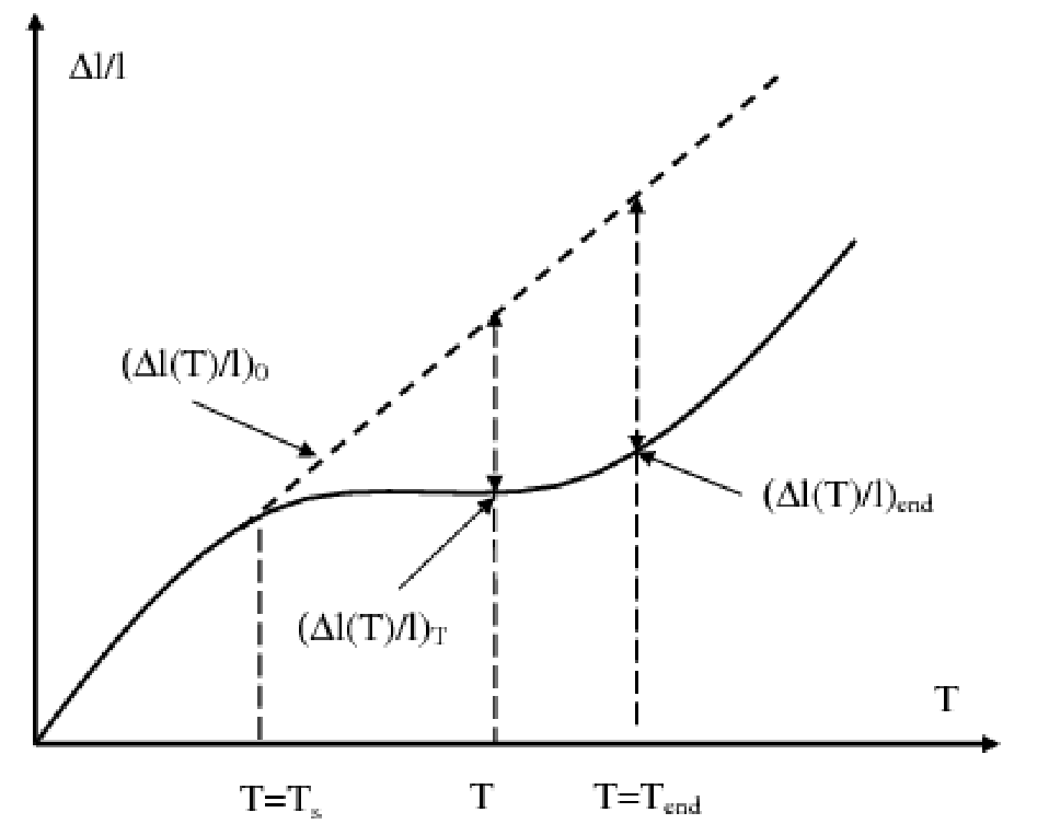
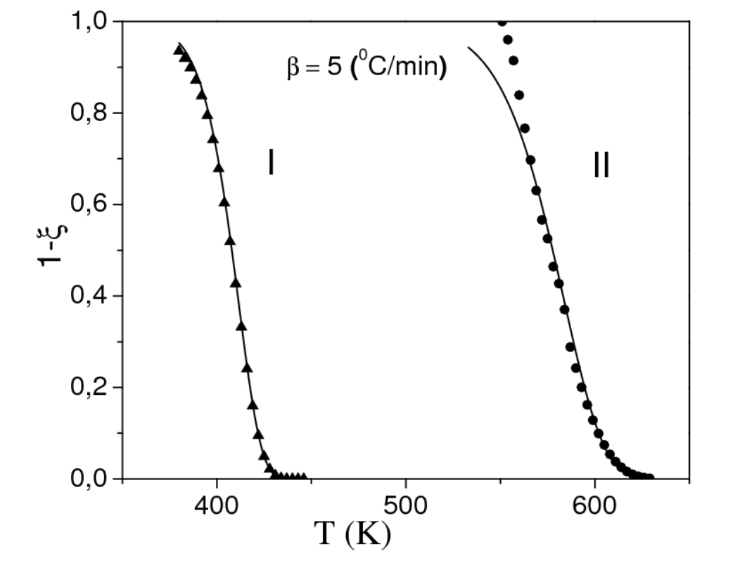
Calculating the fraction untransformed across the whole temperature range, using the fitted values, and plotting it against the experimental points is the check on the whole set. The two curves in Fig. 9 follow the points through both bands. The study notes that other nucleation and growth protocols, which produce a different value of n0, generate visible deviations between the calculated and experimental curves over the temperature range where the reactions actually develop, so the fit is sensitive to that choice.
What the numbers mean in a tempering furnace
Three practical points follow from the parameters above. The two tempering reactions are separated in temperature by roughly 170 K at these heating rates, which is why a single hold at a temperature below about 400 °C does only the first reaction, and why the second needs either a higher temperature or a long hold. The apparent activation energy of the second reaction, near 200 kJ/mol, is high enough that its rate changes sharply with temperature, so a 20 K change in the tempering set point moves it much more than it moves the first reaction. That is the quantitative reason a furnace that is 20 K off its set point still produces a usable tool when the temper is a low temperature one, and produces a large spread in hardness when the temper is being run to form cementite.
The second point concerns the measurement itself. Every number on this page was extracted from the change in length of a specimen, and the resolution of that measurement sets the noise in the fraction transformed, which in turn sets the uncertainty on the exponent. The uncertainties printed in Tables 13 to 15 are calculated from a length resolution of 10-4 and a temperature uncertainty of 0.1 K, so a laboratory reading a dilatometer with a poorer resolution would return wider bounds on the same steel rather than a different mechanism.
The third point is about what the kinetic parameters are not. They describe two reactions in a low alloy steel and in AISI 1050, not the secondary hardening that a molybdenum or vanadium bearing tool steel develops at higher tempering temperatures, which is a third reaction with its own kinetics and its own temperature range. For a tool steel, the tempering response that matters is the secondary hardening peak, and the hardness a given grade reaches at a given temperature is plotted on the tool steel tempering chart.
Source: Alloy Steel, Properties and Use, InTech, 2011.