
X-Ray Diffraction Residual Stress Measurement in Tool Steel
Residual stress decides whether a hardened tool holds its size, whether a ground surface is safe, and whether a die cracks at a corner that looked sound. It is also the property most often quoted from a single measurement, taken at one spot, with a technique and an elastic constant that the person reading the report cannot see. This page covers what the x-ray diffraction method actually measures on a hardened tool steel, which radiation and which peak are used, why the elastic constant scales the answer, how the surface layer is stepped down, and what the method exposes about grinding that a nital etch and a hardness check both miss.
Stress is never measured, strain is
Every method of stress determination measures something else and calculates the stress from it. In x-ray diffraction the measured quantity is the spacing of a set of crystal lattice planes, which changes when the lattice is elastically strained. The angle at which the beam diffracts follows Bragg’s law, so any change in lattice spacing shows up as a shift in the diffraction angle. Lattice spacing is measured in at least two known orientations of the sample relative to the beam, and the stress is calculated from the change between them, assuming linear elastic distortion of the lattice.
The lattice spacing is what the diffractometer actually reads, and the geometry that relates one to the other is the Bragg relation.
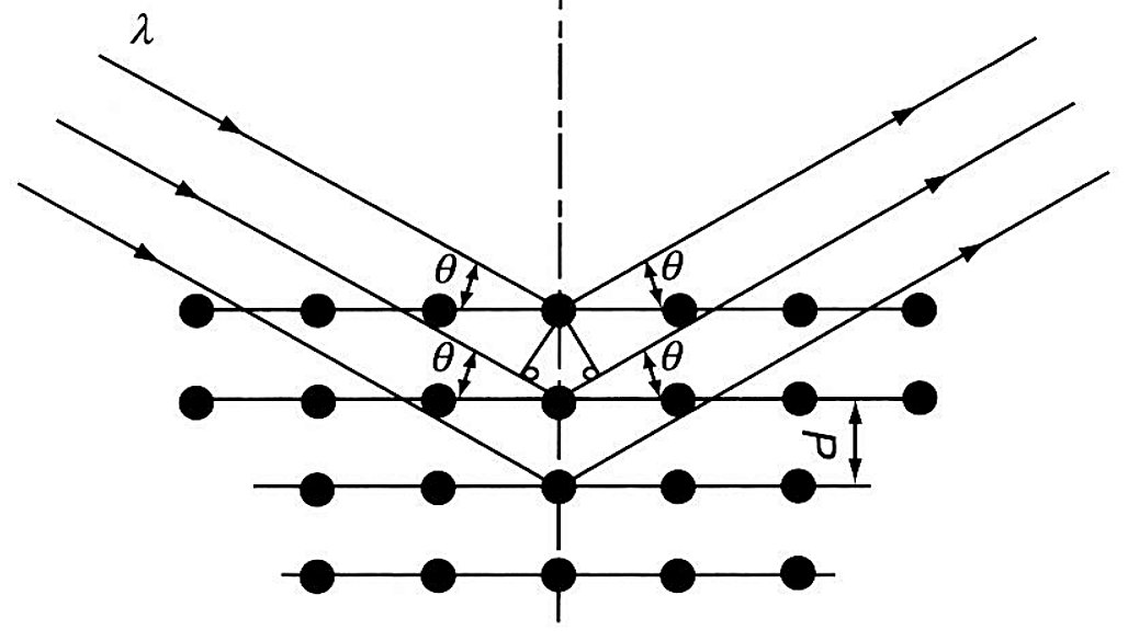
Two consequences follow from that, and both matter when a number is being argued over. First, only elastic strain changes the mean lattice spacing, so the method reports elastic strain only. Once the elastic limit is passed, further straining moves dislocations and disrupts the lattice instead of raising the macroscopic stress, which is why a heavily cold worked surface can carry a stress above the yield strength of the same steel in the annealed condition. Second, the result is an average over a volume, and that volume is set by the size of the irradiated area and by how deep the beam goes. In iron, nickel and aluminium base alloys, half of the diffracted radiation comes from a layer about 0.005 mm deep, which is the reason the method resolves a depth profile that no mechanical or ultrasonic method can approach.
The same scan gives two different things. A macro stress, which extends over distances large relative to the grain size, shifts the position of the diffraction peak. A micro stress, which is the scalar condition behind cold work and hardness, broadens it. Peak position and peak breadth are read from the same measurement, so a properly reported result can carry a stress figure and a cold work or hardness figure together.
Which radiation and which peak
Precision improves with the diffraction angle, so practical work needs a peak above about 120 degrees 2θ. In practice that narrows the choice to a few combinations. On hardened ferrous alloys the standard technique is chromium Kα radiation on the (211) planes, which puts the peak at about 155 to 156 degrees 2θ. On austenitic stainless and nickel base alloys the usual choice is copper Kα on the (420) planes at about 146 to 148 degrees.
Radiation selection also runs into fluorescence. Copper Kα on an alloy containing iron, chromium or titanium produces a fluorescent background several times more intense than the diffracted beam itself, which destroys the signal to noise ratio the peak location depends on. Foil filters help in some cases, and a crystal monochromator or a solid state detector removes the problem, but the position sensitive detectors used for fast stress work are gas filled or screen type and cannot separate the fluorescence out. On a tool steel this is one practical reason the chromium technique dominates.
The elastic constant scales the answer
The stress is proportional to the x-ray elastic constant used, and that constant is not the bulk modulus of the alloy. It belongs to the specific crystallographic direction whose planes are being measured, and because most metals are elastically anisotropic it can differ from the handbook value by tens of percent. The constant is measured empirically by loading a coupon of the actual alloy in four point bending and recording how the lattice spacing moves with applied stress.
The table below is the reason a stress report should state the alloy it was measured on. Taking the bulk value instead of the measured one puts a systematic proportional error of between 7 and 19 percent into the answer on the ferrous alloys listed, and the article puts the worst case across all alloys at 40 percent. A reading quoted to three significant figures while the elastic constant carries a 19 percent uncertainty is a reading quoted to a precision it does not have.
| Alloy and condition | Radiation and plane (hkl) | Diffraction angle 2θ, deg | Measured E/(1 + ν), GPa | Bulk E/(1 + ν), GPa | Difference, % | K45, MPa |
|---|---|---|---|---|---|---|
| 410 stainless, 22 HRC | Cr Kα (211) | 155.1 | 176.5 ± 0.7 | 155.8 | −11.7 | 680 |
| 410 stainless, 42 HRC | Cr Kα (211) | 155.1 | 173.1 ± 1.4 | 155.8 | −9.9 | 667 |
| 1050 carbon steel, 56 HRC | Cr Kα (211) | 156.0 | 184.1 ± 2.1 | 148.2 | −19.4 | 683 |
| 4340 alloy steel, 50 HRC | Cr Kα (211) | 156.0 | 168.9 ± 2.8 | 156.5 | −7.3 | 627 |
| 52100 bearing steel | Cr Kα (211) | 156.0 | 173.7 ± 2.1 | 153.8 | −11.5 | 645 |
| M50 high speed steel, 62 HRC | Cr Kα (211) | 154.0 | 179.3 ± 2.1 | 157.9 | −11.9 | 724 |
| 17-4 PH stainless | Cr Kα (211) | 155.0 | 180.0 ± 0.7 | 158.9 | −11.9 | 696 |
| 304L stainless | Cu Kα (420) | 147.0 | 157.2 ± 2.8 | 151.0 | −3.9 | 814 |
| 316 stainless | Cu Kα (420) | 146.5 | 132.4 ± 1.4 | 153.8 | +16.0 | 696 |
X-ray elastic constants measured in four point bending against the bulk value for the same alloy, with the stress needed to shift the diffraction peak by 1 degree at a 45 degree tilt. Source, Table 1 of X-Ray Diffraction Residual Stress Techniques, in ASM Handbook, Volume 10.
The table also carries a sensitivity column. K45 is the stress required to shift the peak by one degree at a 45 degree tilt, so a larger value means a less sensitive technique. Chromium Kα on (211) sits between about 627 and 724 MPa across these steels, and the copper Kα techniques on the austenitic grades sit in the same band, which is what allows the method to resolve the stress levels that matter on a hardened part.
Getting below the surface
Depth profiling is done by removing material and re-measuring, and the only acceptable way to remove it is electropolishing. Every mechanical method deforms the surface and induces its own residual stress, whatever abrasive or cutting tool is used, so grinding or machining a layer off and then measuring destroys the thing being measured. Where a thick layer has to come off, the article’s rule is to machine or grind most of it and then electropolish at least 0.2 mm to take the damage away.
Two corrections then have to be applied, and skipping either one is where a profile goes wrong. The beam is attenuated exponentially as it enters and leaves the sample, so a measurement made on a surface that sits on top of a steep gradient returns a weighted average rather than the stress at that surface. Where the gradient changes sharply, as it does under a ground surface, the correction can reach 345 MPa. The second correction accounts for the fact that removing a stressed layer lets the remaining material relax, and on an induction hardened shaft where the whole case came off, that correction reached 550 MPa at the maximum depth.
| Source of error | Magnitude | When it applies |
|---|---|---|
| Instrument alignment or sample positioning | about 14 MPa (2 ksi) | An error of 0.025 mm (0.001 in.) at a high diffraction angle, growing rapidly as the angle falls |
| Uncorrected subsurface stress gradient | up to 345 MPa (50 ksi) | A machined or ground surface where the stress changes sharply within the depth the beam penetrates |
| Uncorrected layer removal relaxation | up to 550 MPa (80 ksi) | Removal of the whole hardened case from a 16 mm (0.625 in.) diameter 1070 steel shaft |
| X-ray elastic constant taken from the bulk value | proportional, 7 to 19 % on the ferrous alloys above, up to 40 % in general | Every alloy whose lattice is elastically anisotropic, which is most of them |
| Grain size coarser than ASTM No. 1 | measurement not reliable | Coarse cast structure, where too few crystals diffract to shape a clean peak |
| Partial Kα doublet separation | apparent non-linearity in the d against sin²ψ plot | Peaks that split while the sample is tilted, common in annealed and lightly worked steel |
The error sources worth knowing about before a stress number is quoted as a fact. Compiled from the article text.
Grinding burn is where the method earns its keep
The clearest case in the article is a set of 4340 samples at 50 HRC, two ground abusively to provoke burn and one ground gently with adequate coolant. The difference in the reading is not a matter of degree. The gently ground surface was uniformly in compression at roughly minus 400 to minus 520 MPa. One abusively ground sample was in tension across its entire width, from plus 275 to plus 825 MPa. The other was mixed, and the visible grinder burn sat exactly on the tensile peaks. When the same surface was then read with one large irradiated area, the result came back as about the arithmetic average of the small area readings, which is to say the burn was averaged out of existence by the size of the beam.
| Sample and condition | Longitudinal surface stress, MPa | What was found |
|---|---|---|
| Ground gently, adequate coolant | −400 to −520 | Uniform compression at every point examined |
| Ground abusively, sample A | +275 to +825 | Tension across the whole width, which is the condition for a burn |
| Ground abusively, sample B | mixed, tensile peaks above about +275 | Visible grinder burn sat on the tensile peaks, with compression elsewhere |
| The same surface read with a 13 mm (0.5 in.) wide beam | about the average of the small area results | The wide beam averages the burn away, so the burn disappears from the reading |
Surface stress on three 4340 steel samples at 50 HRC, measured with a 0.5 mm wide beam and then with a 13 mm wide beam. Source, Example 3 of X-Ray Diffraction Residual Stress Techniques, in ASM Handbook, Volume 10.
Two practical warnings come with that. A single surface reading, or a nital etch used to reveal burn, can both miss a subsurface tensile layer that will shorten the life of the tool, because the burn is not always visible and the surface measurement is not always taken where the burn is. On tool steel, where a grinding burn on a die face or a punch is the difference between a tool that runs and a tool that chips, the useful specification is the irradiated area and the number of points, written down next to the result. Our own notes on how far grinding practice can be pushed, and what a burnt surface looks like once it has been cut open, sit in tool steel grindability and grinding wheel selection and in the white layer left by EDM.
Alignment, grain size and peak fitting
Because the lattice strain is small, the peak position has to be located to about 0.01 degrees, and the whole alignment has to be good enough to support that. An alignment or positioning error of 0.025 mm puts about 14 MPa of systematic error into the answer at a high diffraction angle and grows quickly as the angle falls. The check is a loosely compacted stress free powder, which should read within about plus or minus 14 MPa, and the procedure is covered by ASTM E915. Grain size also sets a limit. Coarse grains send too few crystals into the beam and the peak becomes asymmetrical, which shows up as random error, so rocking the sample a few degrees about the tilt axis is used to bring more crystals into diffraction, which extends the workable range to about ASTM grain size 1.
Peak location deserves a mention because it is a hidden variable between laboratories. The chromium Kα radiation used for steel is a doublet, and the two lines blend differently depending on hardness. A fully annealed sample gives a heavily blended, nearly symmetrical peak, while a fully hardened or cold worked sample gives a broad one, and a partly separated doublet appears at intermediate states and when the sample defocuses during tilting. Fitting a parabola to the top of the peak is adequate on a symmetrical profile and can mislead on a partly split one, so the more careful laboratories fit a Pearson VII distribution to the two lines separately. Two laboratories can therefore report different stresses from identical data purely because of the peak fitting method.
The same scan also reports hardness
Peak breadth tracks the microstress in the lattice, and on a hardened steel the microstress tracks hardness closely enough to be used as a measurement. The article gives the curve for M50 high speed steel, where the breadth at half height of the (211) peak was calibrated against Rockwell C hardness. A depth profile can then carry both curves at once, which is what makes the technique useful on a case hardened or induction hardened part where the case is thin, the hardness changes quickly with depth, and a normal hardness traverse cannot resolve it. The same principle is behind the microindentation side of the subject, which is covered in microindentation hardness testing of tool steel.
What this means on a tool steel order
A residual stress figure is only as good as the four things that travel with it, which are the radiation and peak used, the elastic constant and whether it was measured on the alloy or taken from a bulk table, the depth and area the reading represents, and the peak fitting method. Where a customer is qualifying a heat treat cycle or investigating a cracking problem, those four items are worth asking for, and the answer to a cracking complaint usually sits in the depth profile rather than in the surface value. The wider set of ways a measurement reports something other than what was assumed is covered in measuring residual stress in tooling, the crack that follows a bad quench is dealt with in quench cracking in tool steel, and the way the same stress redistributes during a normal heat treat is in tool steel distortion. Grade families with their own heat treat practice are collected under cold work, hot work and high speed tool steels, and where a grade still has to be chosen, the route is how to select tool steels.
Before you act on a stress reading
A reference page, it is not an Aobo Steel specification, and the figures above are the values published for the specific alloys and samples named. A residual stress result belongs with its radiation and lattice plane, its elastic constant, its irradiated area, its depth and the peak fitting method used. A surface value read with a large beam can average a local defect away, and it cannot see a subsurface tensile layer. Ask for the depth profile and the measurement conditions before a stress figure goes into an acceptance decision.
Source: ASM Handbook, Volume 10, Materials Characterization, ASM International, 1986.